Mastering Matrices in R

Clemens Jarnach

2023-03-27

Published in "Level Up Coding" by gitconnected.com

#R #Mathematics

Image by Joshua Sortino on Unsplash

An Introduction to Matrices for Data Manipulation and Analysis

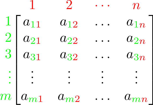
A matrix is a two-dimensional array that contains elements of the same data type (e.g., numeric, character, or logical). In R, matrices can be created using the matrix() function, which takes a vector of elements and specifies the number of rows and columns. Matrices are a fundamental data structure in R, offering immense power and flexibility to perform complex mathematical operations with ease. Matrices in R can store different types of data, from integers and real numbers to characters and even logical values. With built-in functions for basic arithmetic, matrix algebra, and linear algebra, matrices offer a wide range of applications in science, engineering, and finance. In this brief guide, we will explore the basics of matrices in R, how to create and manipulate them, and how to perform mathematical operations on them.

Image by m x n matrix: the m rows are horizontal and the n columns are vertical. Wikimedia

Let's start by creating a basic matrix called my_matrix with three rows and three columns, containing the numbers 1 to 9 in order:

# Create a 3x3 matrix
                        my_matrix <- matrix(c(1, 2, 3, 4, 5, 6, 7, 8, 9), 
                        nrow = 3, ncol = 3)
                        
                        # Print the matrix
                        print(my_matrix)

In this example, we first create a vector with the values 1 through 9 using the c() function. We then pass this vector to the matrix() function, along with the nrow() and ncol() arguments to specify the number of rows and columns in the matrix. Finally, we assign the resulting matrix to the variable my_matrix. The resulting matrix has 3 rows and 3 columns, with the values 1 to 9 arranged in row-major order. We can access individual elements of the matrix using square brackets, like this:

# Get the value in the first row and second column
                        my_matrix[1, 2]  # In our example, this returns 4
                        `

We can also access entire rows or columns of the matrix using the colon operator, like this:

# Get the first row
                        my_matrix[1, ]
                        `

Addition and Subtraction

Built-in R functions allow us to perform matrix operations such as addition, multiplication, and inversion. Let me give you an example of how to perform some basic matrix operations in R. Let's start simple with additions and subtractions:

# First, create two new matrices
                        matrix_A <- matrix(c(1, 2, 3, 4), nrow = 2)
                        matrix_B <- matrix(c(5, 6, 7, 8), nrow = 2)
                        
                        # Matrix addition
                        matrix_C <- matrix_A + matrix_B
                        matrix_C
                        
                        # Matrix subtraction
                        matrix_D <- matrix_B - matrix_A
                        matrix_D

In the example above, we create two 2x2 matrices (matrix_A and matrix_B). We then perform a matrix addition by simply adding the two matrices together to get matrix_C. Similarly, we perform a subtraction to obtain matrix_D. A-OK. That wasn't too hard, was it?

Scalar Multiplication

Next is scalar multiplication, which is the multiplication of each entry in a matrix by the same number; this number is called the 'scalar'. In R, this could look like this:

# Scalar multiplication
                        print( 2 * matrix_B )

Matrix Multiplication

Scalar multiplication is easy. Matrix multiplication, however, is a completely different story. In fact, it's a pain in the neck. But luckily we have R and she does all the calculations for us. Matrix multiplication is the process of multiplying one matrix by another. Matrix multiplication is a mathematical operation performed between two matrices to create a new matrix. It involves multiplying the corresponding elements in each row of the first matrix with the corresponding elements in each column of the second matrix and then summing the results to get the element of the resulting matrix. The number of columns in the first matrix must be equal to the number of rows in the second matrix. If the matrices do not meet this requirement, matrix multiplication cannot be performed. (If you need more information on this read this Wikipedia article on matrix multiplication.) Fortunately, we have R to do all that for us. And here is how:

# Matrix multiplication
                        matrix_E <- matrix_A %*% matrix_B
                        matrix_E

The %*% operator is used to multiply matrices that satisfy the condition that the number of columns in the first matrix is equal to the number of rows in the second matrix. If this condition is not met, R will throw an error indicating that the matrices are not conformable. So far we have added, subtracted, and even multiplied matrices, but what about divisions? WARNING: You cannot divide matrices! There is, however, a related concept called 'inversion'.

Inverse of a Matrix

In linear algebra, the inverse of a matrix is a matrix that, when multiplied by the original matrix, results in an identity matrix. An identity matrix is a square matrix in which all the elements of the main diagonal are 1, and all other elements are 0. Simple! The inverse of a matrix can be calculated only for square matrices. If a matrix A has an inverse, it is denoted as $A^{-1}$. The inverse matrix satisfies the property that $A \times A^{-1} = A^{-1} \times A = I$, where I is the identity matrix. So let's find the inverse of our matrix_A using R:

# Matrix inversion
                        inverse_matrix <- solve(matrix_A)
                        inverse_matrix

We use the solve() function, which is R's standard function for matrix inverse calculations. The solve() function takes a matrix as an argument and returns the inverse of that matrix. The inverse of a matrix has a number of useful applications in linear algebra and related fields, including solving systems of linear equations, calculating determinants, and finding solutions to matrix equations.

apply()function

Another slightly more advanced method for matrices in R is to use the apply() function. This allows you to apply a function to each row or column of a matrix. The apply() function is useful when you need to apply a function to each row or column of a matrix and return a vector or array of the results. The syntax of the apply() function looks like this: apply(X, MARGIN, FUN, ...) where X is the matrix, MARGIN specifies whether the function should be applied to rows (MARGIN=1) or columns (MARGIN=2) of the matrix, FUN is the function to apply, and … indicated that there are more optional arguments possible. Here is an example that uses the apply() function to calculate the row means of a matrix:

# create a 3x4 matrix
                        matrix_F <- matrix(1:12, nrow = 3, ncol = 4)
                        
                        # calculate the row means
                        row_means <- apply(matrix_F, 1, mean)
                        
                        # print the row means
                        row_means

We can also use the apply() function to perform more complex operations on the rows or columns of a matrix. For example, we can calculate the standard deviation of each column of a matrix using the following code:

# create a 4x4 matrix with random numbers 
                        matrix_G <- matrix(rnorm(16), nrow = 4, ncol = 4)
                        matrix_G
                        
                        # calculate the standard deviations for each column
                        column_SD <- apply(matrix_G, 2, sd)
                        
                        # print the column standard deviations
                        column_SD

The first line of code generates a 4x4 matrix named matrix_G. The matrix is created by calling the matrix() function in R, which creates a matrix with random numbers generated by the rnorm() function. The arguments nrow() and ncol() specify the number of rows and columns in the matrix. Just like we did before. This time, the resulting matrix matrix_G will contain 4 rows and 4 columns. The second line of code calculates the standard deviation (SD) of each column of matrix_G using the apply() function in R.

To sum up

Matrices are a mathematical workhorse with extraordinary capabilities in R programming. Their versatility in storing different forms of data allows for simple yet complex mathematical operations. R's matrix() function provides an easy way to create matrices by specifying the number of rows and columns using a vector of elements. Whether in arithmetic, matrix algebra or linear algebra, matrices are widely used in science, engineering and finance.

Resources

R - Matrices: https://www.tutorialspoint.com/r/r_matrices.htm
Wikipedia - Matrix multiplication: https://en.wikipedia.org/wiki/Matrix_multiplication
Wikipedia - Invertible matrix: https://en.wikipedia.org/wiki/Invertible_matrix#Methods_of_matrix_inversion
R - apply(): https://www.rdocumentation.org/packages/base/versions/3.6.2/topics/apply
R - Matrix Inversion: https://www.rdocumentation.org/packages/base/versions/3.6.2/topics/solve
statmethods - Matrix Algebra: https://www.statmethods.net/advstats/matrix.html

• • •

Now it's your turn

You can find a Jupyter notebook of this file, including the R code, on my GitHub page: matrices-in-r.ipynb

👉👈 Follow me for more: Medium | Twitter | GitHub