# Define required packages
want <- c("data.table", "fixest", "ggiraph", "gt", "here", "leaflet",
"lubridate", "janitor", "purrr", "readxl", "scales",
"sf", "tidyverse")
# Check which packages need installing
have <- want %in% rownames(installed.packages())
# Install missing packages
if (any(!have)) install.packages(want[!have])
# Load all packages
junk <- lapply(want, library, character.only = TRUE)
# Clean up
rm(have, want, junk)2 Methods - Visualising Elections
Note
Code Availability: The complete R script used to generate the results shown in the section “1 Results - Elections Visualised” is available as analysis.R in the project’s GitHub repository. This tutorial provides a step-by-step walkthrough of that analysis workflow.
Why geospatial analysis?
Political change is spatial. Electoral outcomes are shaped by place — communities, demographics, and identities linked to geography. Mapping makes these shifts legible, bringing together:
- data science
- visual communication
- political analysis
- reproducibility and open research
This project illustrates how spatial analytics can enrich research in political sociology and public policy.
It demonstrates how to analyse and visualise UK General Election results from 2010-2024 using R. You’ll learn to work with electoral data, create spatial visualisations, and produce both static and interactive maps showing political change across constituencies.
What You’ll Learn
- Loading and cleaning electoral data from Excel files
- Standardising constituency identifiers across different boundary systems
- Creating time-series visualisations of seat counts and vote shares
- Joining electoral data to geographic shapefiles
- Producing choropleth maps showing election results
- Building interactive maps with Leaflet
Data Context: Constituency Boundaries
UK parliamentary constituency boundaries have been revised periodically:
- 1997, 2005, 2010: Major boundary reviews implemented
- 2024: Latest boundary changes for the 2024 election
Important: Elections from 2010-2019 use the 2021 constituency boundaries for consistency. The 2024 election uses updated 2024 boundaries. This means historical results are projected onto current boundaries for visual comparison.
The data uses different identifier codes: - 1997-2001: PCA codes - 2005: Mixed (PCA for England/Wales/NI; ONS for Scotland) - 2010-2019: ONS codes - 2024: ONS codes (new boundaries)
Data Sources
- House of Commons Library: Historical election results (1918-2024)
- ONS: Constituency boundary shapefiles (Dec 2021 and July 2024)
Setup
Install and Load Required Packages
Visualisation 1: Seat Distribution Over Time
This line chart shows how seat counts have changed across elections.
seat_counts_plot <- ggplot(seat_counts,
aes(x = election, y = seats,
color = party, group = party)) +
geom_line(linewidth = 1.2, alpha = 0.9) +
geom_point(size = 4, alpha = 0.9) +
geom_point(size = 2.5, color = "white") + # White center
# Add value labels
geom_text(aes(label = seats),
vjust = -1.2,
size = 3.5,
fontface = "bold",
show.legend = FALSE) +
# Styling
scale_color_manual(
values = party_colors,
name = "Party",
labels = c("Conservative", "Labour", "Liberal Democrats", "SNP")
) +
scale_x_continuous(breaks = c(2010, 2015, 2017, 2019, 2024)) +
scale_y_continuous(limits = c(0, 450), breaks = seq(0, 450, 50)) +
# Labels
labs(
title = "UK General Election Results: Seat Distribution 2010-2024",
subtitle = "The dramatic shift from coalition to Conservative dominance to Labour's 2024 landslide",
x = "Election Year",
y = "Number of Seats",
caption = "Data: House of Commons Library | 650 total seats"
) +
# Theme
theme_minimal(base_size = 12) +
theme(
plot.title = element_text(face = "bold", size = 16, margin = margin(b = 5)),
plot.subtitle = element_text(size = 11, color = "grey40", margin = margin(b = 15)),
plot.caption = element_text(color = "grey50", size = 9, hjust = 0),
panel.grid.minor = element_blank(),
panel.grid.major.x = element_blank(),
legend.position = "top",
legend.title = element_text(face = "bold"),
plot.margin = margin(15, 15, 15, 15)
)
seat_counts_plot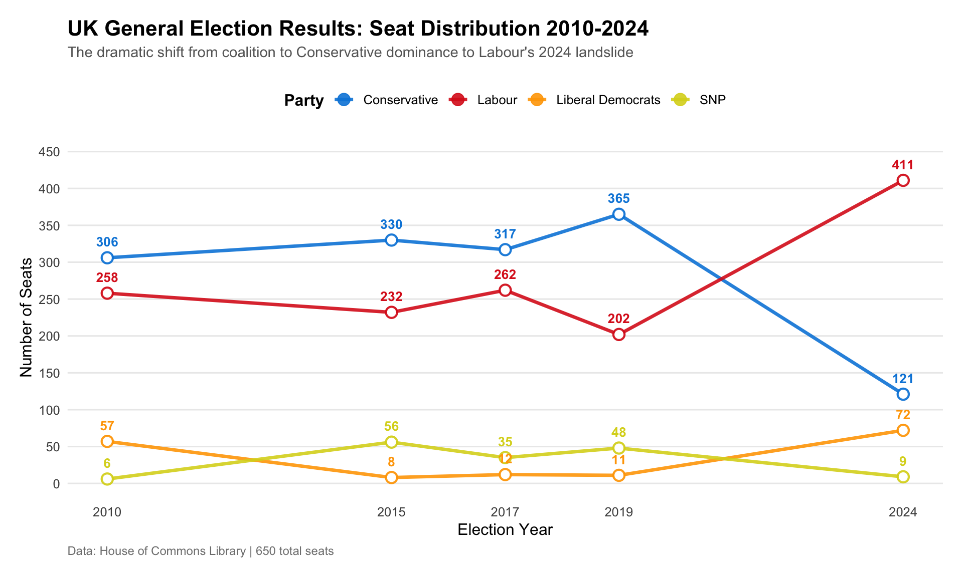
Visualisation 2: Vote Share Over Time
Vote share tells a slightly different story than seats due to the first-past-the-post system.
# Extract vote share data
vote_share_data <- seats_table %>%
select(election, party, vote_share)
# Create visualisation
vote_share_plot <- ggplot(vote_share_data,
aes(x = election, y = vote_share,
color = party, group = party)) +
geom_line(linewidth = 1.2, alpha = 0.9) +
geom_point(size = 4, alpha = 0.9) +
geom_point(size = 2.5, color = "white") +
# Add percentage labels
geom_text(aes(label = paste0(round(vote_share, 1), "%")),
vjust = -1.2,
size = 3.5,
fontface = "bold",
show.legend = FALSE) +
scale_color_manual(
values = party_colors,
name = "Party",
labels = c("Conservative", "Labour", "Liberal Democrats", "SNP")
) +
scale_x_continuous(breaks = c(2010, 2015, 2017, 2019, 2024)) +
scale_y_continuous(
limits = c(0, 70),
breaks = seq(0, 70, 10),
labels = function(x) paste0(x, "%")
) +
labs(
title = "UK General Election Results: Vote Share 2010-2024",
subtitle = "First-past-the-post distortion: vote share tells a different story than seats",
x = "Election Year",
y = "Vote Share (%)",
caption = "Data: House of Commons Library"
) +
theme_minimal(base_size = 12) +
theme(
plot.title = element_text(face = "bold", size = 16, margin = margin(b = 5)),
plot.subtitle = element_text(size = 11, color = "grey40", margin = margin(b = 15)),
plot.caption = element_text(color = "grey50", size = 9, hjust = 0),
panel.grid.minor = element_blank(),
panel.grid.major.x = element_blank(),
legend.position = "top",
plot.margin = margin(15, 15, 15, 15)
)
vote_share_plot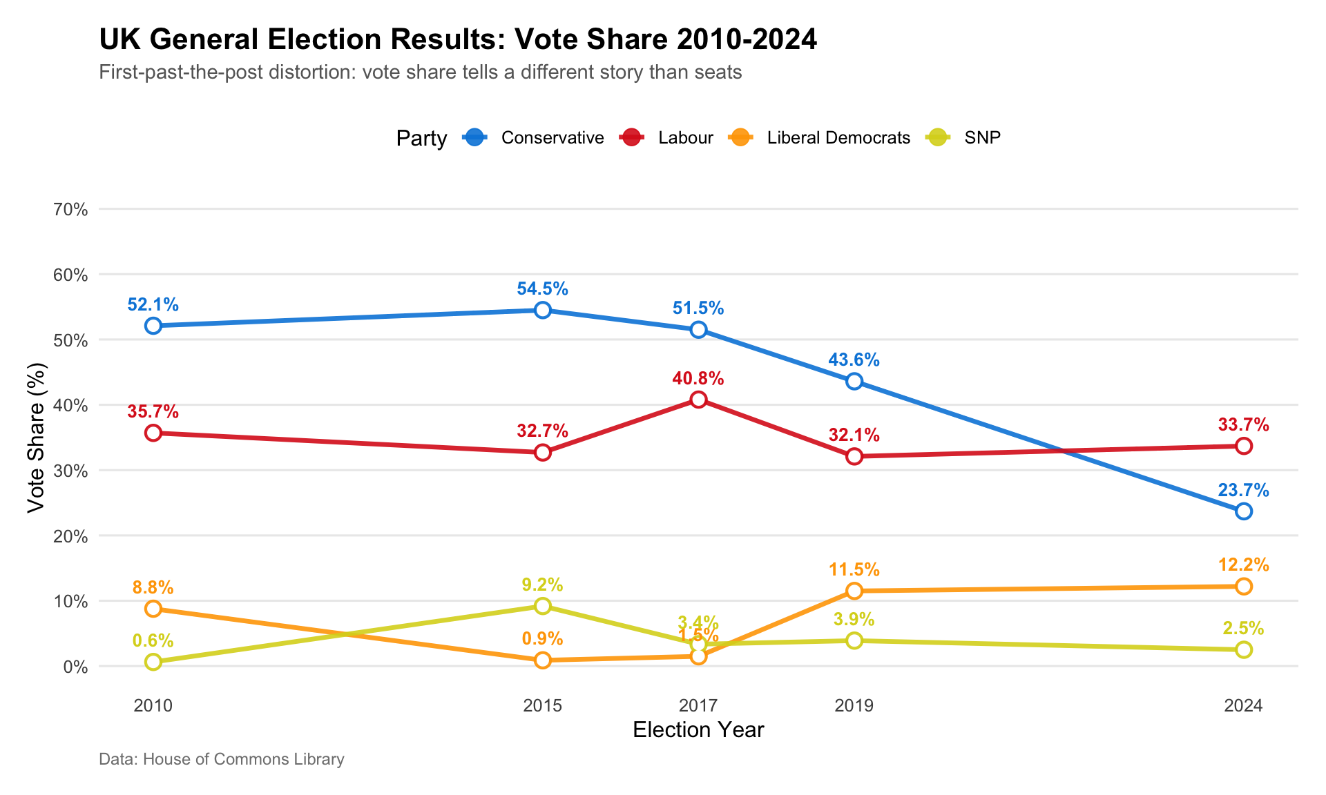
Visualisation 3: Bar Charts by Election
Bar charts provide a clear snapshot of each individual election.
Create a Reusable Function
create_election_bar <- function(year) {
data_year <- seat_counts %>% filter(election == year)
ggplot(data_year, aes(x = party, y = seats, fill = party)) +
geom_col(width = 0.7, alpha = 0.9) +
geom_text(aes(label = seats),
vjust = -0.5,
size = 5,
fontface = "bold") +
scale_fill_manual(values = party_colors) +
scale_y_continuous(limits = c(0, 650), breaks = seq(0, 650, 50)) +
labs(
title = paste0(year, " General Election Results"),
subtitle = "Total seats won by major parties (650 seats total)",
x = NULL,
y = "Number of Seats",
caption = "Data: House of Commons Library"
) +
theme_minimal(base_size = 14) +
theme(
plot.title = element_text(face = "bold", size = 18, hjust = 0.5),
plot.subtitle = element_text(size = 12, color = "grey40", hjust = 0.5),
legend.position = "none",
panel.grid.major.x = element_blank(),
panel.grid.minor = element_blank(),
axis.text.x = element_text(size = 12, face = "bold")
)
}Generate Plots for Each Election
plot_2010 <- create_election_bar(2010)
plot_2015 <- create_election_bar(2015)
plot_2017 <- create_election_bar(2017)
plot_2019 <- create_election_bar(2019)
plot_2024 <- create_election_bar(2024)
# Display (2019 as example)
plot_2019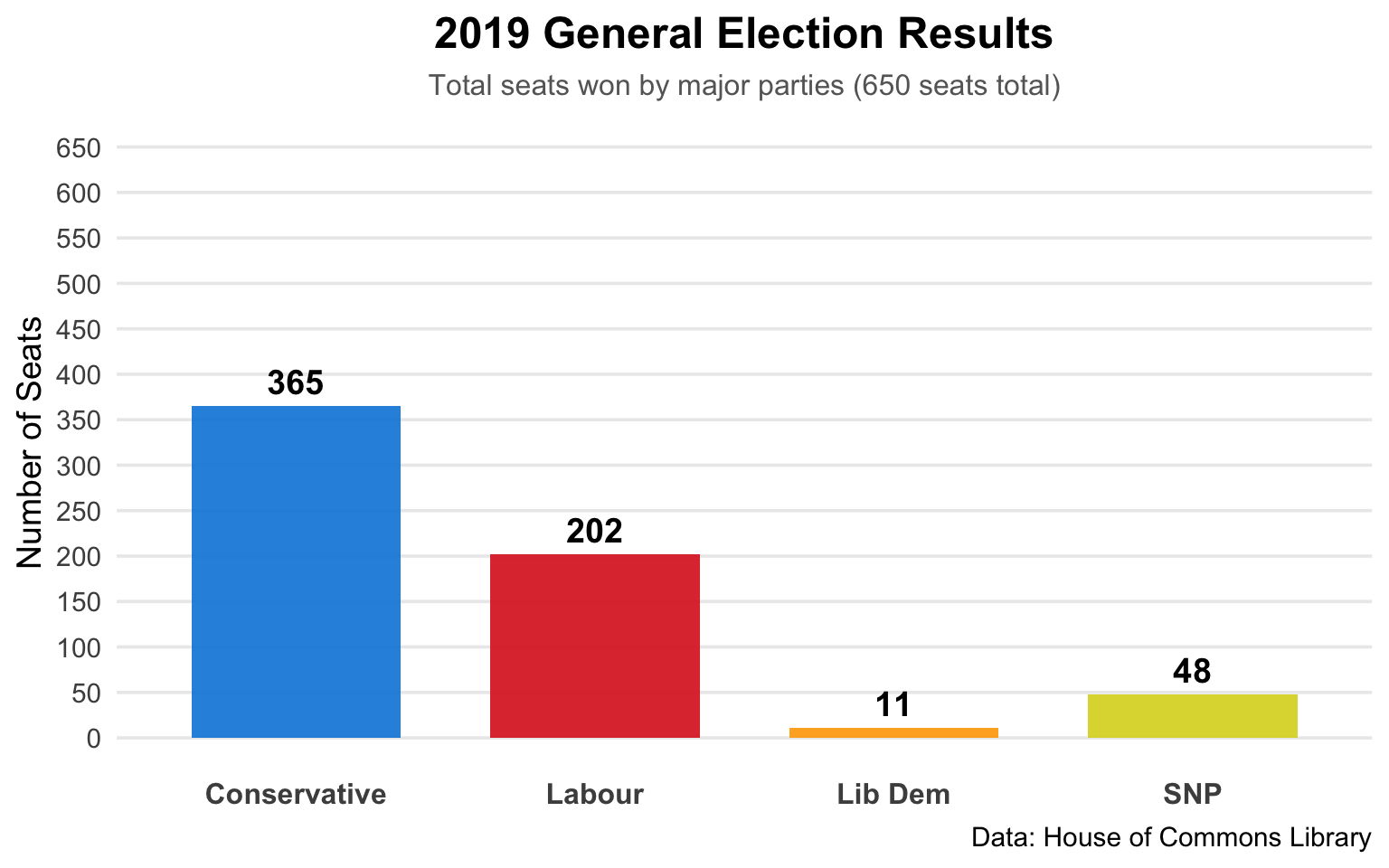
Visualisation 4: Interactive Bar Charts
We can make these charts interactive using ggiraph, allowing users to hover over bars for details.
create_election_bar_interactive <- function(year) {
data_year <- seat_counts %>%
filter(election == year) %>%
mutate(
tooltip = paste0(party, ": ", seats, " seats\n(", year, ")"),
data_id = party
)
p <- ggplot(data_year, aes(x = party, y = seats, fill = party)) +
geom_col_interactive(
aes(tooltip = tooltip, data_id = data_id),
width = 0.7,
alpha = 0.9
) +
geom_text(aes(label = seats), vjust = -0.5, size = 5, fontface = "bold") +
scale_fill_manual(values = party_colors) +
scale_y_continuous(limits = c(0, 650), breaks = seq(0, 650, 50)) +
labs(
title = paste0(year, " General Election Results"),
subtitle = "Total seats won by major parties (650 total)",
x = NULL,
y = "Seats",
caption = "Data: House of Commons Library"
) +
theme_minimal(base_size = 14) +
theme(
plot.title = element_text(face = "bold", size = 18, hjust = 0.5),
plot.subtitle = element_text(size = 12, color = "grey40", hjust = 0.5),
legend.position = "none",
panel.grid.major.x = element_blank()
)
girafe(
ggobj = p,
options = list(
opts_hover(css = "fill:black;"),
opts_hover_inv(css = "opacity:0.5;"),
opts_tooltip(css = "background:#222;color:white;padding:6px;border-radius:4px;")
)
)
}
# Create interactive plot
plot_i_2024 <- create_election_bar_interactive(2024)
plot_i_2024Part 2: Spatial Analysis - Constituency-Level Maps
Now we’ll move to constituency-level data to create choropleth maps.
Load Detailed Election Data (2010-2019)
file <- here::here("data", "1918-2019election_results_by_pcon.xlsx")
# Define target years
target_years <- c("2010", "2015", "2017", "2019")
# Function to read and clean each sheet
read_hoc_sheet <- function(sheet) {
raw <- readxl::read_excel(
file,
sheet = sheet,
skip = 3,
col_names = TRUE
) %>%
janitor::clean_names()
# Identify party vote columns
vote_cols <- grep("_votes$", names(raw), value = TRUE)
# Select core columns and add election year
raw %>%
select(id, constituency, electorate, total_votes, turnout,
all_of(vote_cols)) %>%
mutate(election = as.integer(sheet))
}
# Read all target years
data_wide <- purrr::map_dfr(target_years, read_hoc_sheet)
# Remove empty rows
data_wide <- data_wide %>% filter(!is.na(id))Standardising Constituency Codes
Some constituencies have multiple IDs. We prioritise ONS codes (starting with letters) for consistency.
# Create constituency-to-ID mapping
constituency_pairs_df <- data_wide %>%
select(id, constituency) %>%
unique()
# Prioritise ONS codes
unique_constituency_map_prioritized <- constituency_pairs_df %>%
mutate(is_ons_code = str_detect(id, "^[A-Za-z]")) %>%
arrange(desc(is_ons_code)) %>%
group_by(constituency) %>%
slice_head(n = 1) %>%
ungroup() %>%
select(-is_ons_code)
# Update data with standardised IDs
data_wide <- data_wide %>%
left_join(
unique_constituency_map_prioritized,
by = "constituency",
suffix = c("_old", "")
)Pivot to Long Format
Convert from wide format (one column per party) to long format (one row per party per constituency).
data <- data_wide %>%
pivot_longer(
cols = matches("(votes$|votes_share$)"),
names_to = c("party", ".value"),
names_pattern = "(.*)_(votes|votes_share)$"
) %>%
rename(
ons_code = id,
vote_share = votes_share
) %>%
filter(party != "total") %>%
select(ons_code, constituency, election, party, votes, vote_share, everything()) %>%
select(-id_old)
# Verify structure
data %>%
filter(ons_code == "W07000049", election == 2019) %>%
head()# A tibble: 6 × 8
ons_code constituency election party votes vote_share electorate
<chr> <chr> <int> <chr> <dbl> <dbl> <dbl>
1 W07000049 ABERAVON 2019 conse… 6518 0.206 50750
2 W07000049 ABERAVON 2019 liber… 1072 0.0339 50750
3 W07000049 ABERAVON 2019 labour 17008 0.538 50750
4 W07000049 ABERAVON 2019 ukip NA NA 50750
5 W07000049 ABERAVON 2019 green 450 0.0142 50750
6 W07000049 ABERAVON 2019 snp NA NA 50750
# ℹ 1 more variable: turnout <dbl>Load Geographic Data
# Load pre-processed shapefile
uk_const_2021 <- readRDS(
here("data", "processed", "uk_constituencies_2021_simplified.rds")
)
# Rename to match our data
uk_const <- uk_const_2021 %>%
rename(ons_code = pcon21cd)Note: The shapefile has been pre-processed and simplified to reduce file size. Original source: ONS December 2021 boundaries.
Identify Winners by Constituency
# Find winning party in each constituency for each election
winners <- data %>%
group_by(election, ons_code) %>%
slice_max(votes, n = 1, with_ties = FALSE) %>%
ungroup()
# Join to geographic data
map_df <- uk_const %>%
left_join(winners, by = "ons_code")Define Party Colours for Maps
party_cols <- c(
"conservative" = "#0087DC",
"labour" = "#DC241f",
"liberal_democrats" = "#FDBB30",
"snp" = "#FFFF00",
"plaid_cymru" = "#005B54",
"green" = "#52C152",
"brexit" = "#12B6CF",
"reform_uk" = "#00B5E2",
"ukip" = "#6D3177",
"independent" = "grey60",
"dup" = "#D46A4C",
"sinn_fein" = "#326760",
"sdlp" = "#2AA82C",
"uup" = "#48A5EE",
"alliance" = "#F6CB2F",
"other" = "grey80"
)Create Static Choropleth Maps
# Function to create map for any year
create_static_map <- function(year) {
map_df %>%
filter(election == year) %>%
ggplot(aes(fill = party)) +
geom_sf(colour = "white", linewidth = 0.1) +
scale_fill_manual(values = party_cols, na.value = "grey90") +
theme_minimal() +
labs(
title = paste0(year, " UK General Election"),
subtitle = "Winning party by constituency",
fill = "Party"
) +
theme(
plot.title = element_text(face = "bold", size = 14),
plot.subtitle = element_text(size = 11, color = "grey40")
)
}
# Generate maps
map_2010 <- create_static_map(2010)
map_2019 <- create_static_map(2019)
# Display
map_2010
map_2019
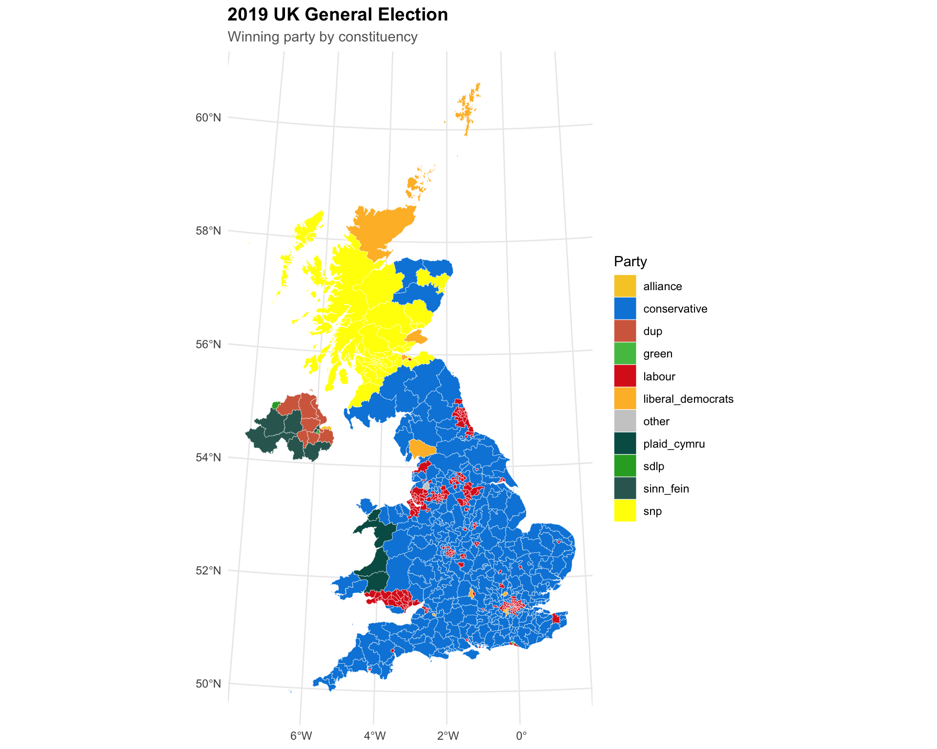
Spatial Patterns
Notice how: - Scotland shifted from Labour (2010) to SNP (2015+) - “Red Wall” constituencies in Northern England flipped Conservative (2019) - Urban centres remained Labour strongholds - Liberal Democrats hold scattered rural/suburban seats
Create Interactive Maps with Leaflet
Interactive maps allow users to explore individual constituencies.
create_interactive_map <- function(election_year) {
# Filter and transform data
map_year <- map_df %>%
filter(election == election_year) %>%
st_transform(4326) # Web Mercator for Leaflet
# Create colour palette
pal <- colorFactor(
palette = party_cols,
domain = map_year$party,
levels = names(party_cols)
)
# Build leaflet map
leaflet(map_year) %>%
addProviderTiles(providers$CartoDB.Positron) %>%
addPolygons(
fillColor = ~pal(party),
fillOpacity = 0.7,
color = "white",
weight = 0.5,
opacity = 1,
highlight = highlightOptions(
weight = 2,
color = "#666",
fillOpacity = 0.9,
bringToFront = TRUE
),
label = ~paste0(pcon21nm, ": ", party),
popup = ~paste0(
"<strong>", pcon21nm, "</strong><br/>",
"Party: ", party, "<br/>",
"Votes: ", format(votes, big.mark = ","), "<br/>",
"Vote Share: ", round(vote_share, 1), "%"
),
labelOptions = labelOptions(
style = list("font-weight" = "normal", padding = "3px 8px"),
textsize = "13px",
direction = "auto"
)
) %>%
addLegend(
position = "bottomright",
pal = pal,
values = ~party,
title = paste(election_year, "Winner"),
opacity = 0.7
)
}
# Create interactive map for 2019
map_interactive_2019 <- create_interactive_map(2019)
map_interactive_2019Part 3: The 2024 Election (New Boundaries)
The 2024 election uses new constituency boundaries, requiring separate processing.
Load 2024 Data
# Read 2024 results
data_wide_2024 <- readxl::read_excel(
here::here("data", "1918-2019election_results_by_pcon.xlsx"),
sheet = "2024",
skip = 3,
col_names = TRUE
) %>%
janitor::clean_names() %>%
filter(!is.na(id)) %>%
select(id, constituency, electorate, total_votes, turnout,
ends_with("_votes")) %>%
mutate(
election = 2024L,
across(
ends_with("_votes"),
~ .x / total_votes,
.names = "{.col}_share"
)
)
# Standardise IDs
data_wide_2024 <- data_wide_2024 %>%
group_by(constituency) %>%
slice_min(order_by = !str_detect(id, "^[A-Za-z]"), n = 1, with_ties = FALSE) %>%
ungroup() %>%
rename(ons_code = id)
# Pivot to long format
data_2024 <- data_wide_2024 %>%
pivot_longer(
cols = ends_with(c("_votes", "_votes_share")),
names_to = c("party", ".value"),
names_pattern = "(.*)_(votes|votes_share)$"
) %>%
rename(vote_share = votes_share) %>%
filter(party != "total") %>%
select(ons_code, constituency, election, party, votes, vote_share, everything())Load 2024 Boundaries
# Load pre-processed 2024 boundaries
uk_const_2024 <- readRDS(
here("data", "processed", "uk_constituencies_2024_simplified.rds")
)
# Identify winners
winners_2024 <- data_2024 %>%
group_by(ons_code) %>%
slice_max(votes, n = 1, with_ties = FALSE) %>%
ungroup()
# Join to geography
map_df_2024 <- uk_const_2024 %>%
left_join(winners_2024, by = "ons_code")Interactive 2024 Map
# Transform for web mapping
map_df_2024_web <- map_df_2024 %>% st_transform(4326)
# Create colour palette
pal_2024 <- colorFactor(
palette = party_cols,
domain = map_df_2024_web$party,
levels = names(party_cols)
)
# Build interactive map
map_interactive_2024 <- leaflet(map_df_2024_web) %>%
addProviderTiles(providers$CartoDB.Positron) %>%
addPolygons(
fillColor = ~pal_2024(party),
fillOpacity = 0.7,
color = "white",
weight = 0.5,
opacity = 1,
highlight = highlightOptions(
weight = 2,
color = "#666",
fillOpacity = 0.9,
bringToFront = TRUE
),
label = ~paste0(pcon24nm, ": ", party),
popup = ~paste0(
"<strong>", pcon24nm, "</strong><br/>",
"Party: ", party, "<br/>",
"Votes: ", format(votes, big.mark = ","), "<br/>",
"Vote Share: ", round(vote_share, 1), "%"
)
) %>%
addLegend(
position = "bottomright",
pal = pal_2024,
values = ~party,
title = "Winning Party",
opacity = 0.7
)
map_interactive_2024References
House of Commons Library (2024). General Election Results, 1918-2024. Retrieved from https://commonslibrary.parliament.uk/research-briefings/cbp-8647/
Office for National Statistics (2021, 2024). Westminster Parliamentary Constituencies Boundaries. Available via Open Geography Portal.
Session Info
sessionInfo()R version 4.1.2 (2021-11-01)
Platform: x86_64-apple-darwin17.0 (64-bit)
Running under: macOS 26.0.1
Matrix products: default
BLAS: /Library/Frameworks/R.framework/Versions/4.1/Resources/lib/libRblas.0.dylib
LAPACK: /Library/Frameworks/R.framework/Versions/4.1/Resources/lib/libRlapack.dylib
locale:
[1] en_US.UTF-8/en_US.UTF-8/en_US.UTF-8/C/en_US.UTF-8/en_US.UTF-8
attached base packages:
[1] stats graphics grDevices utils datasets methods
[7] base
other attached packages:
[1] forcats_1.0.0 stringr_1.5.1 dplyr_1.1.4
[4] readr_2.1.5 tidyr_1.3.1 tibble_3.2.1
[7] ggplot2_3.5.2 tidyverse_2.0.0 sf_1.0-12
[10] scales_1.3.0 readxl_1.4.4 purrr_1.0.1
[13] janitor_2.2.1 lubridate_1.9.4 leaflet_2.2.3
[16] here_1.0.1 gt_1.1.0 ggiraph_0.8.7
[19] fixest_0.12.1 data.table_1.17.0
loaded via a namespace (and not attached):
[1] jsonlite_1.9.1 splines_4.1.2
[3] Formula_1.2-5 cellranger_1.1.0
[5] yaml_2.3.10 numDeriv_2016.8-1.1
[7] pillar_1.10.1 lattice_0.22-6
[9] glue_1.8.0 uuid_1.2-1
[11] digest_0.6.37 snakecase_0.11.1
[13] leaflet.providers_2.0.0 colorspace_2.1-1
[15] sandwich_3.1-1 htmltools_0.5.8.1
[17] Matrix_1.5-1 pkgconfig_2.0.3
[19] xtable_1.8-4 mvtnorm_1.1-3
[21] tzdb_0.4.0 timechange_0.3.0
[23] emmeans_1.10.7 proxy_0.4-27
[25] farver_2.1.2 generics_0.1.3
[27] withr_3.0.2 TH.data_1.1-3
[29] cli_3.6.5 survival_3.8-3
[31] magrittr_2.0.3 estimability_1.5.1
[33] evaluate_1.0.3 fs_1.6.5
[35] nlme_3.1-162 MASS_7.3-54
[37] xml2_1.4.0 class_7.3-23
[39] dreamerr_1.4.0 tools_4.1.2
[41] hms_1.1.3 lifecycle_1.0.4
[43] multcomp_1.4-28 munsell_0.5.1
[45] jquerylib_0.1.4 compiler_4.1.2
[47] e1071_1.7-16 systemfonts_1.0.4
[49] rlang_1.1.6 classInt_0.4-9
[51] units_0.8-2 grid_4.1.2
[53] rstudioapi_0.17.1 htmlwidgets_1.6.4
[55] crosstalk_1.2.1 rmarkdown_2.29
[57] gtable_0.3.6 codetools_0.2-20
[59] DBI_1.2.3 R6_2.6.1
[61] zoo_1.8-13 knitr_1.49
[63] utf8_1.2.4 fastmap_1.2.0
[65] rprojroot_2.0.4 stringmagic_1.1.2
[67] KernSmooth_2.23-20 stringi_1.8.4
[69] Rcpp_1.0.14 vctrs_0.6.5
[71] tidyselect_1.2.1 xfun_0.51
[73] coda_0.19-4.1