---
title: "Working with Panel Data in R"
subtitle: "Structure, Reshaping, Indexing, and Missingness"
author: "[Dr Clemens Jarnach](https://clemensjarnach.github.io)"
affiliation: "Oxford Martin School, University of Oxford"
date: "04-16-2026"
format:
html:
toc: true
toc-depth: 2
code-fold: false
theme: cosmo
self-contained: false
execute:
warning: false
message: false
---
```{r}
#| label: setup
#| include: false
if (!file.exists("files/panel_data.csv")) {
source("simple_panel_data.r")
}
library(tidyverse)
library(plm)
library(lubridate)
library(knitr)
```
Before estimating any model, we need to understand the two fundamental shapes that panel data can take, know how to move between them, and be able to detect and address the most common data quality problems. This chapter covers all three.
------------------------------------------------------------------------
## Two Shapes of Panel Data
Panel data — repeated observations on the same units over time — can be stored in two distinct formats. Understanding the difference is essential before you can do anything else.
### Person-level (wide) format
In **wide** format, each row represents one unit (a person, firm, or country) and each wave of measurement occupies a separate column. This is how many surveys distribute their data and how non-specialists tend to organise spreadsheets.
```{r}
#| label: wide-example
wide_example <- tibble(
  id     = 1:4,
  gender = c("F", "M", "F", "M"),
  wage_2020 = c(2.1, 3.4, 1.8, 2.9),
  wage_2021 = c(2.3, 3.6, 1.9, 3.1),
  wage_2022 = c(2.4, 3.5, 2.2, 3.3),
  educ_2020 = c(12, 16, 14, 12),
  educ_2021 = c(12, 16, 16, 12),
  educ_2022 = c(14, 16, 16, 14)
)

wide_example
```
Each person appears on exactly **one row**. Repeated measurements are spread across columns named by variable and wave (`wage_2020`, `wage_2021`, …). This makes it easy to compute within-person changes (subtract column A from column B), but it is awkward for modelling: most statistical functions in R expect one observation per row.
### Person-period (long) format
In **long** format, each row is one observation — one unit at one point in time. A person observed at four time points occupies four rows.
```{r}
#| label: long-example
long_example <- wide_example |>
  pivot_longer(
    cols      = starts_with("wage_") | starts_with("educ_"),
    names_to  = c(".value", "year"),
    names_sep = "_"
  ) |>
  mutate(year = as.integer(year))

long_example
```
This is the format required by virtually all panel model packages in R (`plm`, `fixest`, `lme4`). Each row has a unit identifier (`id`), a time identifier (`year`), and then the variables measured at that wave.
::: callout-note
### Which format does your data arrive in?
Survey data is often wide: one row per respondent, with wave-specific suffixes. Administrative records are usually long: each event or measurement is a separate record. Knowing which you have determines your first step.
:::
------------------------------------------------------------------------
## Reading Panel Data into R
### CSV and tabular data
The workshop dataset — 200 individuals tracked annually from 2016 to 2023 — is stored as a CSV:
```{r}
#| label: read-data
panel_data <- read_csv("files/panel_data.csv", show_col_types = FALSE)

glimpse(panel_data)
```
The dataset is already in **long format**: each row is one person-year. The key identifiers are `id` (person) and `year` (time).
### Stata and SPSS files
Many longitudinal datasets are distributed in Stata (`.dta`) or SPSS (`.sav`) format. The `haven` package reads both directly, preserving value labels:
```{r}
#| label: haven-example
#| eval: false
library(haven)

# Stata
df_stata <- read_dta("your_data.dta")

# SPSS
df_spss  <- read_sav("your_data.sav")

# Convert labelled columns to factors
df_stata <- df_stata |> mutate(across(where(is.labelled), as_factor))
```
### Excel files
```{r}
#| label: excel-example
#| eval: false
library(readxl)

df_xl <- read_excel("your_data.xlsx", sheet = "Panel", na = c("", "NA", "."))
```
------------------------------------------------------------------------
## Inspecting the Panel Structure
Before modelling, always verify that your data is what you think it is.
### How many units? How many periods?
```{r}
#| label: structure-check
cat("Individuals :", n_distinct(panel_data$id), "\n")
cat("Time periods:", n_distinct(panel_data$year), "\n")
cat("Total rows :", nrow(panel_data), "\n")
cat("Year range :", min(panel_data$year), "–", max(panel_data$year), "\n")
```
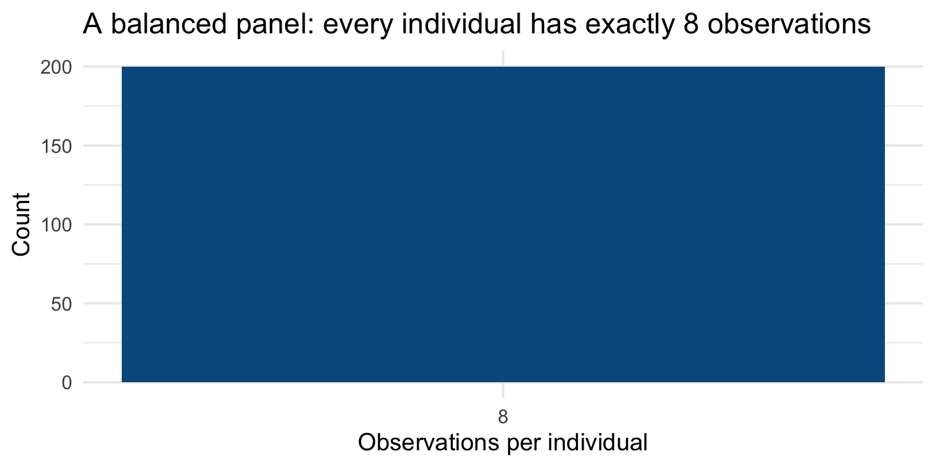
### Is the panel balanced?
A **balanced** panel has the same number of time points for every unit. An **unbalanced** panel does not — some units are observed less frequently. The distinction matters for estimation.
```{r}
#| label: balance-check
obs_per_person <- panel_data |>
  count(id, name = "n_obs")

obs_per_person |>
  count(n_obs, name = "n_individuals") |>
  kable(
    col.names = c("Observations per person", "Number of individuals"),
    caption   = "Table 1 — Panel balance check"
  )
```
```{r}
#| label: balance-plot
#| fig-cap: "Figure 1 — Number of observations per individual (balanced panel)"
#| fig-height: 3.5
ggplot(obs_per_person, aes(x = n_obs)) +
  geom_bar(fill = "#045a8d", width = 0.6) +
  scale_x_continuous(breaks = 1:10) +
  labs(x = "Observations per individual", y = "Count",
       title = "A balanced panel: every individual has exactly 8 observations") +
  theme_minimal(base_size = 13)
```
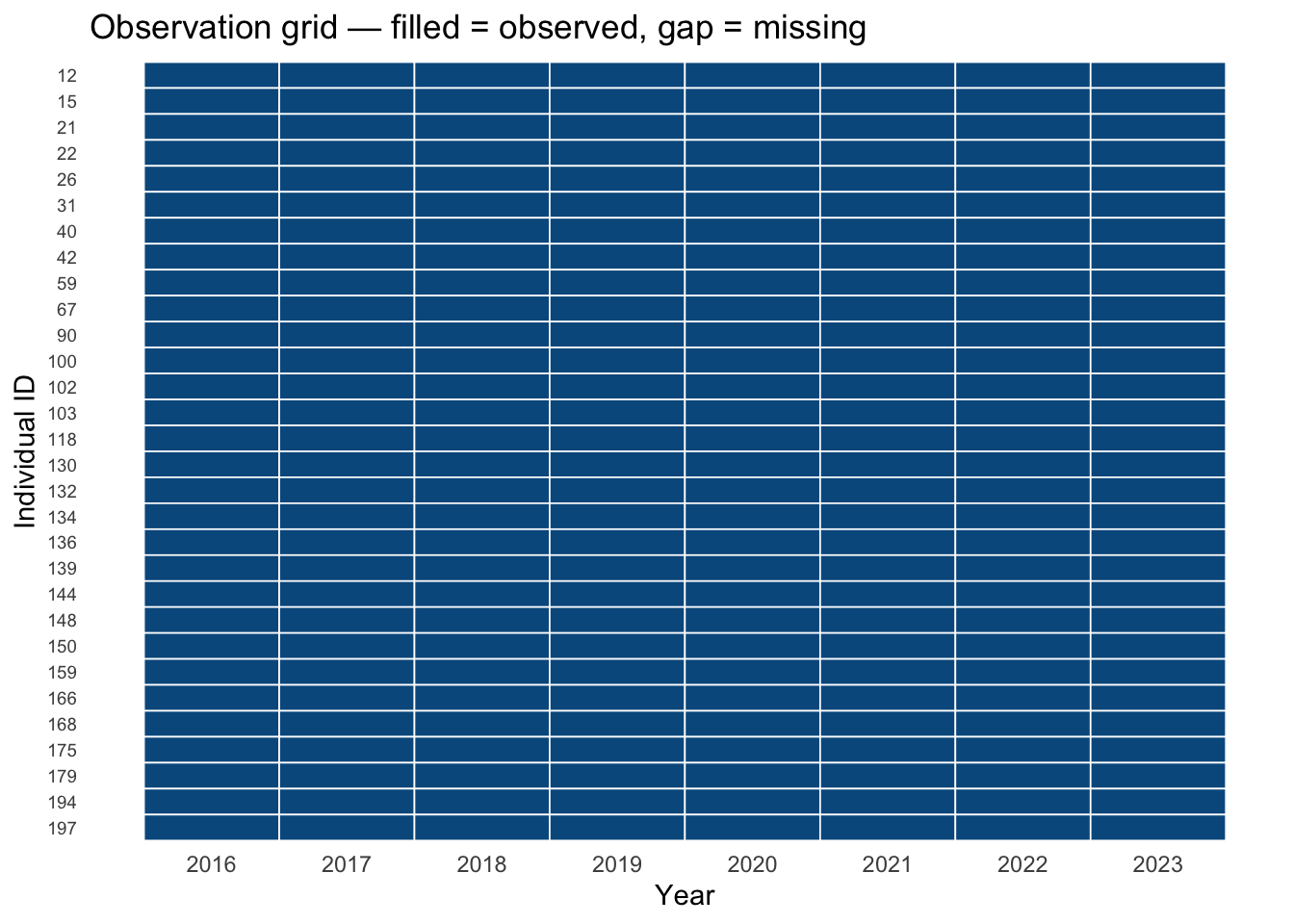
### Unit and time coverage at a glance
For small panels it can be useful to visualise which units are observed at which times — a "swimmer plot" or tile chart that reveals gaps immediately.
```{r}
#| label: coverage-plot
#| fig-cap: "Figure 2 — Observation coverage for a random sample of 30 individuals"
#| fig-height: 5
set.seed(7)
sample_ids <- sample(unique(panel_data$id), 30)

panel_data |>
  filter(id %in% sample_ids) |>
  mutate(id = factor(id, levels = rev(sort(sample_ids)))) |>
  ggplot(aes(x = year, y = id)) +
  geom_tile(fill = "#045a8d", colour = "white", linewidth = 0.3) +
  scale_x_continuous(breaks = 2016:2023) +
  labs(x = "Year", y = "Individual ID",
       title = "Observation grid — filled = observed, gap = missing") +
  theme_minimal(base_size = 11) +
  theme(axis.text.y = element_text(size = 7),
        panel.grid  = element_blank())
```
------------------------------------------------------------------------
## Cleaning Panel Data
### Standardise variable names
The `janitor` package's `clean_names()` converts all column names to `snake_case`, removes special characters, and ensures uniqueness. Get into the habit of calling it immediately after reading data.
```{r}
#| label: clean-names
#| eval: false
# Requires: install.packages("janitor")
library(janitor)

# Simulate messy column names from an external file
messy <- tibble(
  `Person ID` = 1:3,
  `Survey Year` = 2020:2022,
  `Log Wage (£)` = c(7.2, 7.4, 7.3),
  `Union Member?` = c(1, 0, 1)
)

messy |> clean_names()
```
### Parse and handle date variables
Many longitudinal datasets record time as a date string rather than an integer year. `lubridate` provides a consistent grammar for parsing and computing with dates.
```{r}
#| label: lubridate-example
date_example <- tibble(
  id           = c(1, 1, 2, 2),
  interview_dt = c("2020-03-15", "2022-09-01", "2020-06-22", "2022-11-30")
)

date_example <- date_example |>
  mutate(
    interview_dt = ymd(interview_dt),           # parse to Date
    year         = year(interview_dt),          # extract year
    month        = month(interview_dt, label = TRUE),
    wave_gap_days = as.integer(
      interview_dt - lag(interview_dt), units = "days"
    )
  )

date_example
```
### Recode and relabel variables
```{r}
#| label: recode
panel_data <- panel_data |>
  mutate(
    gender    = factor(gender, levels = c("Male", "Female")),
    sector    = factor(sector, levels = c("Public", "Private")),
    union_lbl = if_else(union == 1, "Union member", "Non-member")
  )

panel_data |>
  count(gender, sector) |>
  kable(caption = "Table 2 — Cross-tabulation: gender × sector")
```
------------------------------------------------------------------------
## Reshaping: Wide ↔ Long
### Long to wide with `pivot_wider`
Sometimes you need wide format — for example to compute person-level change scores or to merge with a cross-sectional dataset.
```{r}
#| label: pivot-wider
wages_wide <- panel_data |>
  select(id, year, wage) |>
  pivot_wider(
    names_from  = year,
    values_from = wage,
    names_prefix = "wage_"
  )

head(wages_wide, 5)
```
You can now compute within-person change between any two waves:
```{r}
#| label: change-scores
wages_wide <- wages_wide |>
  mutate(wage_change_16_23 = wage_2023 - wage_2016)

wages_wide |>
  select(id, wage_2016, wage_2023, wage_change_16_23) |>
  slice_head(n = 6) |>
  kable(
    col.names = c("ID", "Wage 2016", "Wage 2023", "Change 2016→2023"),
    caption   = "Table 3 — Within-person wage change (wide format)"
  )
```
### Wide to long with `pivot_longer`
To go back to long format, or when your data arrives wide:
```{r}
#| label: pivot-longer
wages_long_again <- wages_wide |>
  select(id, starts_with("wage_20")) |>      # drop the change score
  pivot_longer(
    cols         = starts_with("wage_20"),
    names_to     = "year",
    names_prefix = "wage_",
    values_to    = "wage"
  ) |>
  mutate(year = as.integer(year))

head(wages_long_again, 8)
```
### Reshaping multiple variables simultaneously
When several variables are wave-stamped (e.g., `wage_2020`, `educ_2020`, `wage_2021`, `educ_2021`), use the `".value"` sentinel in `names_to` to split the column name into variable name and wave:
```{r}
#| label: pivot-multi-var
# Reconstruct a multi-variable wide dataset to demonstrate
multi_wide <- panel_data |>
  select(id, year, wage, education) |>
  filter(id <= 3) |>
  pivot_wider(
    names_from  = year,
    values_from = c(wage, education)
  )

# Pivot back to long, splitting "wage_2016" into variable="wage", year="2016"
multi_wide |>
  pivot_longer(
    cols      = -id,
    names_to  = c(".value", "year"),
    names_sep = "_(?=\\d{4}$)"           # split on _ before a 4-digit year
  ) |>
  mutate(year = as.integer(year)) |>
  arrange(id, year)
```
------------------------------------------------------------------------
## Indexing: Creating a `pdata.frame`
The `plm` package works with **panel data frames** — objects that know which columns identify units and time. Creating one is the gateway to all of `plm`'s modelling and diagnostic functions.
```{r}
#| label: pdata-frame
pdata <- pdata.frame(panel_data, index = c("id", "year"))

# The class is both a pdata.frame and a data.frame
class(pdata)
```
### Inspecting the panel index
```{r}
#| label: pdim
pdim(pdata)
```
`pdim()` reports the panel dimensions and whether it is balanced. The `T` here is the number of time periods, `N` the number of individuals.
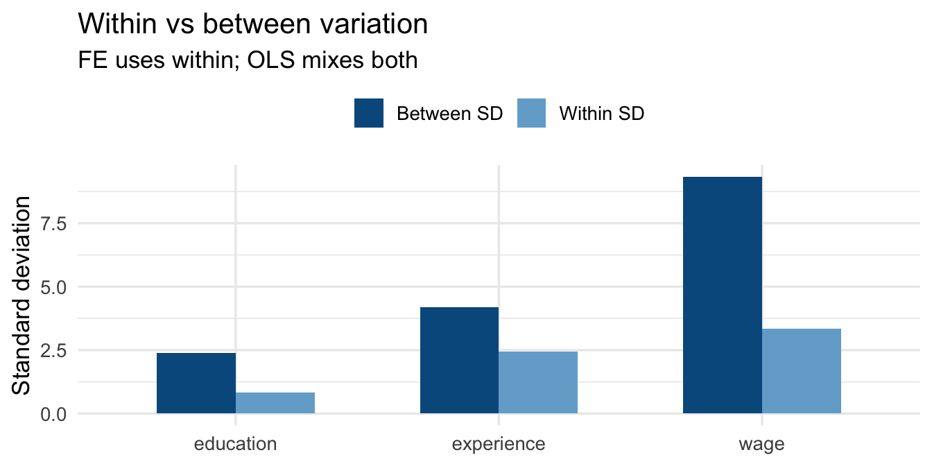
### Within and between variation
A central diagnostic in panel analysis is how much variation in your key variables is *within* units (across time) versus *between* units (across individuals). `plm::Within()` and `between()` compute these directly.
```{r}
#| label: within-between
within_between <- panel_data |>
  summarise(
    across(
      c(wage, education, experience),
      list(
        total_sd  = \(x) round(sd(x, na.rm = TRUE), 3),
        between_sd = \(x) round(sd(tapply(x, id, mean, na.rm = TRUE),
                                  na.rm = TRUE), 3),
        within_sd  = \(x) round(mean(tapply(x, id,
                                  \(v) sd(v, na.rm = TRUE),
                                  simplify = TRUE), na.rm = TRUE), 3)
      )
    )
  ) |>
  pivot_longer(everything(), names_to = c("Variable", ".value"),
               names_sep = "_(?=total|between|within)") |>
  rename(`Total SD` = total_sd,
         `Between SD` = between_sd,
         `Within SD` = within_sd)

kable(within_between,
      caption = "Table 4 — Decomposition of variance: total, between, and within")
```
::: callout-tip
### Reading the variance decomposition
- **Between SD** — how much the *person-average* of a variable varies across individuals. This is the variation exploited by cross-sectional (OLS) models.
- **Within SD** — how much a variable varies *within* the same individual over time. This is the variation used by the Fixed Effects estimator.
A variable with low within-SD and high between-SD (e.g., gender) carries little information for a within-estimator. A variable with high within-SD (e.g., experience) is well-suited to fixed effects analysis.
:::
```{r}
#| label: within-between-plot
#| fig-cap: "Figure 3 — Within vs between standard deviation for key variables"
#| fig-height: 3.5
within_between |>
  pivot_longer(c(`Between SD`, `Within SD`),
               names_to = "Component", values_to = "SD") |>
  ggplot(aes(x = Variable, y = SD, fill = Component)) +
  geom_col(position = "dodge", width = 0.6) +
  scale_fill_manual(values = c("Between SD" = "#045a8d",
                               "Within SD"  = "#74add1")) +
  labs(x = NULL, y = "Standard deviation", fill = NULL,
       title = "Within vs between variation",
       subtitle = "FE uses within; OLS mixes both") +
  theme_minimal(base_size = 13) +
  theme(legend.position = "top")
```
------------------------------------------------------------------------
## Handling Missingness
Real panel datasets almost always have missing values. The source and pattern of missingness determines how seriously it threatens your estimates.
### Types of missingness
| Type | Definition | Implication |
|----|----|----|
| **MCAR** | Missing completely at random — missingness is unrelated to any variable | Listwise deletion is unbiased (just less efficient) |
| **MAR** | Missing at random — missingness depends on *observed* variables | Multiple imputation or FIML can recover unbiased estimates |
| **MNAR** | Missing not at random — missingness depends on the *unobserved* value itself | Requires a selection model; listwise deletion is biased |
### Detecting missingness
```{r}
#| label: missing-summary
missing_summary <- panel_data |>
  summarise(across(everything(),
                   \(x) sum(is.na(x)))) |>
  pivot_longer(everything(),
               names_to  = "Variable",
               values_to = "N missing") |>
  mutate(`% missing` = round(`N missing` / nrow(panel_data) * 100, 2)) |>
  filter(`N missing` > 0)

kable(missing_summary,
      caption = "Table 5 — Missing values by variable")
```
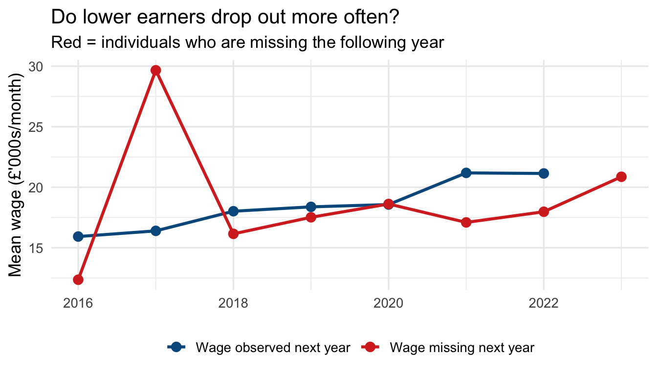
### Is missingness systematic? {#sec-missing-systematic}
The first question to ask: is missingness in the outcome related to observed predictors? If it is, listwise deletion may introduce bias.
```{r}
#| label: missing-pattern
#| fig-cap: "Figure 4 — Mean wage by year and missingness in the following year"
#| fig-height: 4
panel_data |>
  arrange(id, year) |>
  group_by(id) |>
  mutate(
    missing_next_wage = is.na(dplyr::lead(wage))
  ) |>
  ungroup() |>
  filter(!is.na(missing_next_wage)) |>
  group_by(year, missing_next_wage) |>
  summarise(mean_wage = mean(wage, na.rm = TRUE), .groups = "drop") |>
  ggplot(aes(x = year, y = mean_wage,
             colour = missing_next_wage, group = missing_next_wage)) +
  geom_line(linewidth = 1.1) +
  geom_point(size = 3) +
  scale_colour_manual(values = c("FALSE" = "#045a8d", "TRUE" = "#d73027"),
                      labels  = c("Wage observed next year",
                                  "Wage missing next year")) +
  labs(x = NULL, y = "Mean wage (£'000s/month)", colour = NULL,
       title = "Do lower earners drop out more often?",
       subtitle = "Red = individuals who are missing the following year") +
  theme_minimal(base_size = 13) +
  theme(legend.position = "bottom")
```
### Listwise deletion (complete cases)
The default in most R model functions. Observations with any `NA` on the modelled variables are dropped. This is valid only under MCAR.
```{r}
#| label: complete-cases
panel_complete <- panel_data |> drop_na(wage, education, experience, union)

cat("Rows before:", nrow(panel_data),    "\n")
cat("Rows after :", nrow(panel_complete), "\n")
cat("Dropped :", nrow(panel_data) - nrow(panel_complete), "\n")
```
### Carrying observations forward (`fill`)
In some panel datasets, a variable is recorded only when it changes (e.g., a diagnosis or employment status). `tidyr::fill()` propagates the last observed value forward (or backward) within each unit.
```{r}
#| label: fill-example
fill_example <- tibble(
  id     = c(1, 1, 1, 1, 2, 2, 2, 2),
  year   = rep(2020:2023, 2),
  status = c("Employed", NA, NA, "Unemployed",
             "Student",  NA, "Employed", NA)
)

fill_example |>
  group_by(id) |>
  fill(status, .direction = "down") |>
  ungroup()
```
### Checking panel balance after dropping missing rows
Dropping rows due to missingness can **unbalance** a previously balanced panel. Always recheck after listwise deletion:
```{r}
#| label: recheck-balance
pdata_complete <- pdata.frame(panel_complete, index = c("id", "year"))
pdim(pdata_complete)
```
::: callout-warning
### Unbalanced panels and fixed effects
An unbalanced panel is not invalid — `plm` and `fixest` both handle it correctly. But it is worth understanding *why* balance was lost: if high-wage or low-wage individuals are disproportionately missing, your within-estimator still operates on a selected sample.
:::
### Flagging and summarising incomplete spells
::: callout-note
### What is a "spell"?
In the context of longitudinal data and panel studies, a **spell** refers to a continuous period of time that an individual spends in a particular state — employed, unemployed, enrolled in education, living in a given region, and so on.
Think of it as a single "chapter" or "streak" in someone's data: a spell begins when the individual enters a state and ends when they leave it. A person may have multiple spells of the same type over the observation window (e.g., two separate employment spells separated by a period of unemployment).
In the code below, a *complete spell* means an individual is observed in every time period in the dataset — their "chapter" has no missing pages.
:::
```{r}
#| label: incomplete-spells
incomplete <- panel_data |>
  group_by(id) |>
  summarise(
    n_obs   = n(),
    n_miss  = sum(is.na(wage)),
    complete = n_obs == max(panel_data |>
                 count(id) |> pull(n))
  ) |>
  ungroup()

incomplete |>
  count(complete) |>
  mutate(label = if_else(complete, "Complete spells", "Incomplete spells")) |>
  kable(col.names = c("Complete", "N individuals", "Label"),
        caption = "Table 6 — Complete vs incomplete individual spells")
```
------------------------------------------------------------------------
## Summary
| Task | Key function(s) |
|----|----|
| Read CSV / Stata / SPSS / Excel | `read_csv()`, `read_dta()`, `read_sav()`, `read_excel()` |
| Standardise column names | `janitor::clean_names()` |
| Parse dates | `lubridate::ymd()`, `year()`, `month()` |
| Wide → long | `tidyr::pivot_longer()` |
| Long → wide | `tidyr::pivot_wider()` |
| Check balance | `plm::pdim()` |
| Detect missing | `is.na()`, `drop_na()`, `naniar::gg_miss_var()` |
| Carry values forward | `tidyr::fill()` |
| Panel index | `plm::pdata.frame(df, index = c("id", "time"))` |
| Within/between split | `plm::Within()`, `plm::between()` |
::: callout-important
### Before fitting any model, always verify
1. Your data is in **long format** (one row per unit × time).
2. The unit and time **identifiers are correct** and uniquely index each row.
3. The panel is **balanced** — or you understand why it isn't.
4. You know the **direction and magnitude of missingness** in your outcome.
5. You have decomposed key variables into **within and between components** to understand what variation your chosen estimator will exploit.
:::
------------------------------------------------------------------------
## Common Panel Data Sources
Panel and longitudinal datasets come from a wide range of sources. Below is a selection of well-known survey-based panels and process-generated datasets with a longitudinal dimension.
### Household and individual panel surveys
These are purpose-designed surveys that track the same individuals or households over many waves:
- [**PSID**](https://psidonline.isr.umich.edu/) — Panel Study of Income Dynamics (USA); one of the longest-running household panel surveys, covering income, wealth, employment, and health since 1968.
- [**NLSY79**](https://www.nlsinfo.org/content/cohorts/nlsy79) — National Longitudinal Survey of Youth 1979 cohort (USA); tracks labour market experiences, education, and family formation.
- [**Understanding Society**](https://www.understandingsociety.ac.uk/) — UK Household Longitudinal Study; follows \~40,000 households annually on a broad range of social and economic outcomes.
- [**Millennium Cohort Study**](https://cls.ucl.ac.uk/cls-studies/millennium-cohort-study/) — Follows \~19,000 children born in the UK in 2000–01 through childhood, adolescence, and into adulthood.
- [**SOEP**](https://www.diw.de/en/diw_01.c.615551.en/research_infrastructure__socio-economic_panel__soep.html) — Socio-Economic Panel Study (Germany); annual household survey running since 1984, covering income, employment, health, and well-being.
- [**pairfam**](https://www.pairfam.de/) — Panel Analysis of Intimate Relationships and Family Dynamics (Germany); focuses on partnership, fertility, and intergenerational relations.
- [**SHARE**](http://www.share-project.org/home0.html) — Survey of Health, Ageing and Retirement in Europe; multi-country panel of individuals aged 50+.
### Process-generated longitudinal data
Administrative records and monitoring systems often produce data with a natural longitudinal structure, even though they were not designed as surveys:
- [**Our World in Data — COVID-19**](https://github.com/owid/covid-19-data) — Country-day panel of cases, deaths, vaccinations, and policy responses; well-documented and regularly updated.
- [**UK Census (Nomis)**](https://www.nomisweb.co.uk/sources/census) — Area-level statistics from the decennial UK Census; geographic units can be tracked across census years.
- [**London Air Quality Network**](https://data.london.gov.uk/air-quality/) — Station-level time series of pollutant concentrations across London.
- [**Copernicus Tree Cover Density**](https://land.copernicus.eu/pan-european/high-resolution-layers/forests/tree-cover-density/status-maps) — Raster-based estimates of tree cover density across Europe; repeated status maps enable change analysis over time.
### Practical considerations
**Merging across waves.** Many panel datasets are distributed as a separate file per wave (each file is cross-sectional), which must be stacked or merged to create a panel. This is a common and time-consuming step. Some data providers or the research community have published pre-written merge scripts to simplify the process — see for example the [Understanding Society syntax library](https://www.understandingsociety.ac.uk/documentation/mainstage/syntax) or the [SOEP teaching materials](https://www.ls3.soziologie.uni-muenchen.de/studium-lehre/lehrmaterialien/index.html).
**Panel attrition.** Participation in surveys tends to fall over successive waves. Individuals drop out for a variety of reasons — non-contact, refusal, migration, or death — and those who remain may be systematically different from those who leave. If attrition is related to the outcome of interest, estimates based on the surviving sample can be biased. Always check how many units are observed across all waves and consider whether attrition looks random.