# Summary
This workshop introduced the core logic and methods of longitudinal data analysis using R. The sections below provide a brief conceptual recap of the three main modelling approaches covered: OLS, Fixed Effects, and Random Effects.
## 1. Ordinary Least Squares (OLS)
**Equation**
$$y_{it} = \beta_0 + \beta_1 x_{it} + u_{it}$$
- $i$ = individual (person, firm, country)
- $t$ = time
- $u_{it}$ = error term
**Key idea**
OLS ignores the panel structure. It treats all observations as independent.
**Unique features**
- One common intercept $\beta_0$ for all units
- No explicit handling of unobserved individual heterogeneity
- Assumes:
$$\text{Cov}(x_{it}, u_{it}) = 0$$
**Problem in panel data**
If there are unobserved individual effects ($\alpha_i$) that affect $y_{it}$ and are correlated with $x_{it}$, then:
- They get absorbed into $u_{it}$
- → Omitted variable bias
---
## 2. Fixed Effects (FE)
**Equation**
$$y_{it} = \alpha_i + \beta_1 x_{it} + u_{it}$$
- $\alpha_i$ = individual-specific intercept (fixed effect)
**Equivalent (demeaned / "within" form)**
$$y_{it} - \bar{y}_i = \beta_1 (x_{it} - \bar{x}_i) + (u_{it} - \bar{u}_i)$$
**Key idea**
Each unit gets its own intercept, and these intercepts can be correlated with $x_{it}$.
**Unique features**
- Controls for all time-invariant unobserved heterogeneity
- Uses only within-individual variation
- Allows:
$$\text{Cov}(x_{it}, \alpha_i) \neq 0$$
**Consequences**
- Cannot estimate coefficients on time-invariant variables
- More robust than OLS in panel settings
---
## 3. Random Effects (RE)
**Equation**
$$y_{it} = \beta_0 + \beta_1 x_{it} + \alpha_i + u_{it}$$
- $\alpha_i$ = random individual effect
**Error structure (composite error term)**
$$\varepsilon_{it} = \alpha_i + u_{it}$$
Individual-specific effects are captured by this composite error term. Rather than estimating a separate intercept for each unit, RE assumes that individual intercepts are drawn from a random distribution of possible intercepts — meaning $\alpha_i$ is not a fixed parameter but a random variable with some distribution.
**Key assumption**
$$\text{Cov}(x_{it}, \alpha_i) = 0$$
**Key idea**
The individual effect is treated as a random variable, not a fixed parameter.
**Unique features**
- Uses both:
- within variation (like FE)
- between variation (differences across individuals)
- Estimated via GLS (Generalized Least Squares)
- Implicitly applies partial pooling
**Consequences**
- Can estimate time-invariant variables
- More efficient than FE if assumptions hold
- Biased if $\alpha_i$ is correlated with $x_{it}$
---
## Side-by-Side Summary
| Feature | OLS | Fixed Effects | Random Effects |
|---|---|---|---|
| Intercept | Single $\beta_0$ | $\alpha_i$ for each unit | $\beta_0 + \alpha_i$ |
| Unobserved heterogeneity | Ignored | Controlled (fixed) | Modeled (random) |
| $\text{Corr}(x_{it}, \alpha_i)$ | Not allowed | Allowed | Not allowed |
| Variation used | All (naively) | Within only | Within + between |
| Time-invariant variables | Yes | No | Yes |
| Bias risk | High for panel data | Low | Depends on assumption |
---
## Model Comparison: Simpson's Paradox
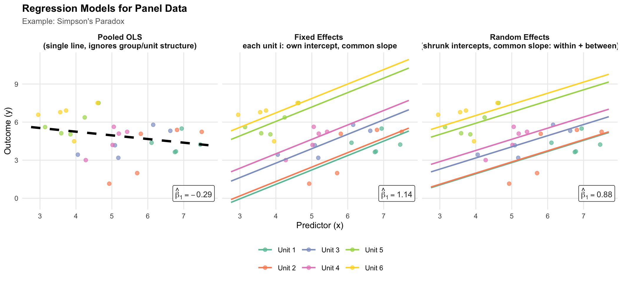
The figure below illustrates how each modelling strategy handles unobserved individual heterogeneity, using a synthetic dataset designed to produce **Simpson's Paradox**: the aggregate (OLS) trend is negative, yet the true within-unit relationship is positive.
Each panel shows the same six simulated units (coloured points). The lines show what each estimator recovers, and each panel is annotated with its slope estimate $\hat{\beta}_1$:
- **OLS** — a single regression line ignoring group membership; the negative between-unit confound dominates.
- **Fixed Effects** — parallel within-unit lines (common slope, unit-specific intercepts); the true positive within-unit relationship is recovered.
- **Random Effects** — GLS estimator that uses a weighted mix of within- and between-unit variation. When $\text{Cov}(x_{it}, \alpha_i) \neq 0$ (as here), the slope is biased toward the OLS estimate — the key trade-off versus FE.
```{r}
#| code-fold: true
#| label: fig-simpsons-paradox
#| fig-cap: "Simpson's Paradox in panel data. OLS recovers the spurious negative aggregate trend; unit-level methods reveal the true positive within-unit relationship. Random Effects partially pools intercepts toward the grand mean relative to FE."
#| fig-width: 11
#| fig-height: 5
#| message: false
#| warning: false
if (!requireNamespace("lme4", quietly = TRUE)) install.packages("lme4")

library(tidyverse)
library(lme4)
library(RColorBrewer)

set.seed(42)

n_units <- 6
n_obs   <- 5   # few obs per unit → θ ≈ 0.70, making RE visibly distinct from FE

# Simpson's paradox: between-unit trend is negative, within-unit trend is positive.
# Smaller unit spread + higher within noise keeps θ well below 1, so RE ≠ FE.
unit_x0 <- seq(6.5, 3.5, length.out = n_units)  # unit mean x (high → low)
unit_y0 <- seq(3.5, 6.5, length.out = n_units)  # unit mean y (low → high)

df <- map_dfr(seq_len(n_units), function(i) {
  x <- unit_x0[i] + rnorm(n_obs, 0, 0.70)
  y <- unit_y0[i] + 0.85 * (x - unit_x0[i]) + rnorm(n_obs, 0, 0.80)
  tibble(unit = factor(paste0("Unit ", i)), x = x, y = y)
})

unit_levels <- levels(df$unit)
xs <- seq(min(df$x) - 0.2, max(df$x) + 0.2, length.out = 80)

# ---- OLS ----
ols_fit   <- lm(y ~ x, data = df)
ols_slope <- as.numeric(coef(ols_fit)["x"])
ols_lines <- tibble(
  x = xs, y = as.numeric(coef(ols_fit)[1]) + ols_slope * xs,
  unit = "Overall", model = "OLS"
)

# ---- Fixed Effects ----
fe_fit   <- lm(y ~ x + unit, data = df)
fe_slope <- as.numeric(coef(fe_fit)["x"])
fe_ints  <- setNames(
  c(coef(fe_fit)["(Intercept)"],
    coef(fe_fit)["(Intercept)"] + coef(fe_fit)[paste0("unit", unit_levels[-1])]),
  unit_levels
)
fe_lines <- map_dfr(unit_levels, function(u) {
  tibble(x = xs, y = as.numeric(fe_ints[u]) + fe_slope * xs, unit = u, model = "Fixed Effects")
})

# ---- Random Effects (random intercept, ML) ----
# With our data, Cov(x_it, α_i) ≠ 0, so RE is biased: its slope will sit between
# the FE slope (within only) and the OLS slope (within + between confounded).
re_fit   <- lmer(y ~ x + (1 | unit), data = df, REML = FALSE)
re_slope <- as.numeric(fixef(re_fit)["x"])
re_int   <- as.numeric(fixef(re_fit)["(Intercept)"])
re_blup  <- data.frame(
  unit = rownames(ranef(re_fit)$unit),
  ran  = ranef(re_fit)$unit[[1]]
)
re_lines <- map_dfr(unit_levels, function(u) {
  ri <- re_blup$ran[re_blup$unit == u]
  tibble(x = xs, y = re_int + ri + re_slope * xs, unit = u, model = "Random Effects")
})

# ---- Combine ----
model_levels <- c("OLS", "Fixed Effects", "Random Effects")

lines_all <- bind_rows(ols_lines, fe_lines, re_lines) %>%
  mutate(model = factor(model, levels = model_levels))

scatter_all <- map_dfr(model_levels, function(m) {
  df %>% mutate(model = factor(m, levels = model_levels))
})

# ---- Slope annotations (one per panel) ----
slope_ann <- tibble(
  model = factor(model_levels, levels = model_levels),
  slope = c(ols_slope, fe_slope, re_slope),
  label = paste0("hat(beta)[1] == ", round(c(ols_slope, fe_slope, re_slope), 2))
)

# ---- Colours ----
unit_colours <- c(
  setNames(brewer.pal(n_units, "Set2"), unit_levels),
  "Overall" = "black"
)

# ---- Plot ----
ggplot() +
  geom_point(
    data = scatter_all,
    aes(x = x, y = y, colour = unit),
    size = 2.0, alpha = 0.70
  ) +
  geom_line(
    data = lines_all %>% filter(unit != "Overall"),
    aes(x = x, y = y, colour = unit),
    linewidth = 0.85
  ) +
  geom_line(
    data = lines_all %>% filter(unit == "Overall"),
    aes(x = x, y = y),
    colour = "black", linewidth = 1.4, linetype = "dashed"
  ) +
  geom_label(
    data  = slope_ann,
    aes(label = label),
    x = Inf, y = -Inf, hjust = 1.08, vjust = -0.5,
    size = 3.6, parse = TRUE,
    fill = alpha("white", 0.85), colour = "grey20", label.size = 0.3
  ) +
  scale_colour_manual(values = unit_colours) +
  facet_wrap(
    ~model, nrow = 1,
    labeller = as_labeller(c(
      "OLS"            = "Pooled OLS\n(single line, ignores group/unit structure)",
      "Fixed Effects"  = "Fixed Effects \neach unit i: own intercept, common slope",
      "Random Effects" = "Random Effects\n(shrunk intercepts, common slope: within + between)"
    ))
  ) +
  labs(
    title    = "Regression Models for Panel Data",
    subtitle = "Example: Simpson's Paradox",
    x      = "Predictor (x)",
    y      = "Outcome (y)",
    colour = NULL
  ) +
  theme_minimal(base_size = 11) +
  theme(
    strip.text       = element_text(face = "bold", size = 10),
    legend.position  = "bottom",
    legend.key.width = unit(1.5, "lines"),
    plot.title       = element_text(face = "bold", size = 13),
    plot.subtitle    = element_text(size = 10, colour = "grey40"),
    panel.grid.minor = element_blank()
  )
```