Appendix
Panel Model Comparison
The figure below illustrates four regression strategies for panel data, all fitted to the same simulated dataset of four groups (shown in different colours). The models differ substantially in how they account for group structure, and consequently in how well they recover the underlying within-group relationship.
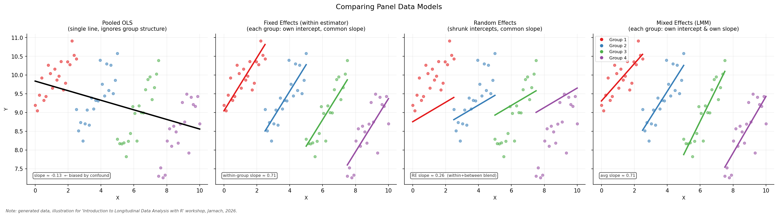
Pooled OLS treats all observations as if they came from a single population, ignoring group membership entirely. When groups differ systematically in both the outcome and the predictor, the resulting slope is confounded and can be severely biased — a classic manifestation of Simpson’s Paradox.
Fixed Effects (FE) addresses this by demeaning within each group (or equivalently, including a group-level intercept for every unit). This removes all time-invariant unobserved heterogeneity, so only within-group variation identifies the slope. It is the primary method covered in this workshop.
Random Effects (RE) assumes that group-level deviations are drawn from a common distribution and are uncorrelated with the predictors. This is a stronger assumption than FE, but it allows time-invariant predictors to be included and can be more efficient when the assumption holds. The Hausman test is the standard tool for choosing between FE and RE.
Mixed Effects (ME) — also called multilevel or hierarchical models — goes one step further by allowing both intercepts and slopes to vary across groups. This is a rich and flexible framework that sits beyond the scope of this introductory workshop.
Presentation Slides
Below are the slides for this module. You can view them in full screen here.
Notation Reference
This appendix provides a quick reference for common mathematical and statistical symbols used throughout the workshop materials, along with their LaTeX commands for use in write-ups and presentations.
| Symbol | LaTeX Command | Common Statistical Use |
|---|---|---|
| α | \alpha |
Significance level / Type I error rate |
| β | \beta |
Regression coefficients / Type II error rate |
| γ | \gamma |
Gamma distribution / Euler-Mascheroni constant |
| δ | \delta |
Small change / Dirac delta function |
| ε | \varepsilon |
Error term (residuals) in regression (variant form) |
| ϵ | \epsilon |
Error term (residuals) in regression |
| μ | \mu |
Population mean |
| π | \pi |
Population proportion / Probability of success |
| ρ | \rho |
Population correlation coefficient |
| σ | \sigma |
Population standard deviation |
| τ | \tau |
Kendall’s Tau / Precision (inverse variance) |
| θ | \theta |
General unknown parameter |
| Σ | \sum |
Summation operator |
| ∏ | \prod |
Product operator |
Dummy Variable Trap
The Dummy Variable Trap is a scenario in which independent variables are highly collinear—specifically, when one variable can be predicted perfectly from the others. In technical terms, it is a case of perfect multicollinearity.
Here is how it happens and how to avoid it.
How the Trap is Set
When you have a categorical variable (like “Gender” or “Season”) and you want to include it in a regression, you create dummy variables (0 or 1).
If you have a category like Season (Spring, Summer, Fall, Winter) and you include a dummy for all four categories plus an intercept (\(\beta_0\)) in your model, you have entered the trap.
The Math Behind the Failure
A standard regression model includes a constant (the intercept), which is essentially a column of 1s. If you add up the values of all your dummy variables for a specific observation, they will always equal 1 (because every observation must belong to exactly one category).
\[Spring + Summer + Fall + Winter = 1\]
Since the sum of your dummies equals your intercept, the computer cannot mathematically distinguish between the effect of the intercept and the combined effect of the dummies. This makes the matrix non-invertible, and your software will either: 1. Crash/return an error. 2. Automatically drop one of the variables.
How to Escape the Trap: The \((n-1)\) Rule
To avoid perfect multicollinearity, you must always include one fewer dummy variable than there are categories.
- If you have 2 categories (Male/Female): Include 1 dummy.
- If you have 4 categories (Seasons): Include 3 dummies.
- If you have 50 cities: Include 49 dummies.
The “Reference” Group
The category you leave out becomes the Reference Group (or Baseline). * If you leave out “Winter,” the coefficients for Spring, Summer, and Fall will represent the difference in the outcome compared to Winter. * The Intercept (\(\beta_0\)) will represent the average value for Winter.
In your previous R code example: lm(crime_rate ~ factor(city)...) R automatically handles this for you by picking the first city (alphabetically) and dropping it to serve as the reference group, effectively saving you from the trap!